CDC and SCD on Apache Iceberg: Patterns, Tradeoffs, and Getting It Right
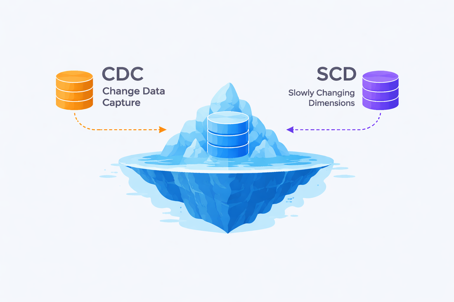
CDC and SCD on Apache Iceberg: Patterns, Tradeoffs, and Getting It Right
Change data capture and slowly changing dimensions are two of the most discussed - and most misunderstood - patterns in data engineering. Every team building an analytical platform eventually has to answer the same questions: how do we track what changed? Do we keep history or just the current state? What happens when events arrive late or out of order?
The tools have evolved significantly. Apache Iceberg in particular changes what's possible: row-level deletes, partition evolution, time travel, and merge-on-read all shift the tradeoff calculus in meaningful ways. But the fundamental design decisions remain hard, and making the wrong call early is expensive to undo.
This post is a technical deep-dive in how to implement CDC and SCD on an Iceberg-based lakehouse with PySpark. I'll cover the core patterns, where each one breaks down, and how Iceberg's table format properties should inform your choices.
First, Get Clear on What You Actually Need
Before choosing a pattern, it's worth being precise about your requirements. The two axes that matter most:
Do you need history?
- No → SCD Type 1 (overwrite in place)
- Yes → SCD Type 2 (append versioned rows)
What is your change source?
- Native CDC stream (Debezium, Kafka Connect, DMS) → work from operation flags (
INSERT,UPDATE,DELETE) - Periodic snapshots (S3 dumps, API exports, batch extracts) → infer changes by diffing successive snapshots
These two axes give you four combinations. Most teams only think about one or two of them upfront, then scramble to retrofit the others later. Design for all four from the start.
SCD Type 1 on Iceberg: Keeping the Current State
SCD Type 1 means your target table always reflects the latest known state of each record. Old values are overwritten. There is no history.
The core operation: MERGE INTO
Iceberg supports MERGE INTO natively via PySpark SQL, and it handles the three cases you need:
spark.sql("""
    MERGE INTO prod.users AS t
    USING (
        SELECT
            user_id,
            name,
            city,
            operation,
            sequence_num,
            ROW_NUMBER() OVER (
                PARTITION BY user_id ORDER BY sequence_num DESC
            ) AS rn
        FROM staging.users_cdc
    ) AS s
    ON t.user_id = s.user_id AND s.rn = 1
    WHEN MATCHED AND s.operation = 'DELETE' THEN DELETE
    WHEN MATCHED AND s.sequence_num > t.sequence_num THEN UPDATE SET
        t.name = s.name,
        t.city = s.city,
        t.sequence_num = s.sequence_num
    WHEN NOT MATCHED AND s.operation != 'DELETE' THEN INSERT *
""")
What breaks here
Out-of-order delivery. The sequence_num > t.sequence_num guard is essential and easy to forget. Without it, a late-arriving event can silently overwrite a newer state. Always carry a sequencing column from the source - a Kafka offset, a database LSN, a timestamp with millisecond precision - and never apply an update unless you can confirm it's newer than what's already in the table.
Deduplication within a micro-batch. If your staging layer contains multiple events for the same key in a single run (common in streaming ingest), a naive MERGE will behave non-deterministically depending on which row the engine processes first. The ROW_NUMBER() window in the example above handles this: deduplicate before merging, not inside the merge condition.
Idempotency on reprocessing. Backfills and retries are inevitable. Your MERGE logic must be safe to run twice on the same data. With a proper sequence guard, reruns are idempotent - the second pass sees sequence_num = sequence_num and skips the update. Test this explicitly; don't assume it.
Iceberg-specific consideration: copy-on-write vs. merge-on-read
Iceberg gives you a choice in how it physically handles row-level updates. This matters at scale.
Copy-on-write (COW): On every write, Iceberg rewrites entire data files that contain changed rows. Reads are fast (no merge needed at query time), but write amplification is high. Works well when updates are infrequent relative to reads, and when updated rows are clustered - e.g., partitioned by updated_date.
Merge-on-read (MOR): Iceberg writes delete files and positional deletes instead of rewriting data files. Writes are cheap; reads merge the base files with the deletes at query time. Works well for high-frequency update workloads. Accumulates read overhead over time until you compact.
# Set write mode per table
spark.sql("""
    ALTER TABLE prod.users
    SET TBLPROPERTIES (
        'write.delete.mode' = 'merge-on-read',
        'write.update.mode' = 'merge-on-read',
        'write.merge.mode' = 'merge-on-read'
    )
""")
For SCD Type 1 with high update rates (fintech transaction states, user profile updates), MOR is almost always the right default. Schedule regular compaction via Iceberg's rewriteDataFiles action to keep read performance from degrading.
SCD Type 2 on Iceberg: Preserving Full History
SCD Type 2 stores every version of a record, with validity windows (effective_from, effective_to) indicating when each version was active. This is the right pattern when you need to answer questions like "what was the customer's address at the time of this transaction?" - a common requirement in fintech and banking.
The data model
user_id | name    | city        | effective_from | effective_to | is_current
--------|---------|-------------|----------------|--------------|----------
123     | Isabel  | Monterrey   | 2025-01-01     | 2025-06-15   | false
123     | Isabel  | Guadalajara | 2025-06-15     | NULL         | true
effective_to = NULL (or a sentinel like 9999-12-31) marks the currently active row. The is_current boolean is optional but speeds up queries significantly.
The two-step write pattern
SCD Type 2 cannot be done in a single MERGE because you need to both close existing rows and insert new ones. The cleanest approach is two operations:
from pyspark.sql import functions as F
from pyspark.sql.window import Window

# Step 1: Load and deduplicate incoming changes
incoming = (
    spark.table("staging.users_cdc")
    .withColumn(
        "rn",
        F.row_number().over(
            Window.partitionBy("user_id").orderBy(F.desc("event_ts"))
        )
    )
    .filter("rn = 1 AND operation != 'DELETE'")
    .drop("rn", "operation")
)

# Step 2: Close currently active rows that are being superseded
(
    spark.table("prod.users_history")
    .alias("t")
    .merge(incoming.alias("s"), "t.user_id = s.user_id AND t.is_current = true")
    .whenMatchedUpdate(set={
        "effective_to": "s.event_ts",
        "is_current": F.lit(False)
    })
    .execute()
)

# Step 3: Insert new versions
(
    incoming
    .withColumn("effective_from", F.col("event_ts"))
    .withColumn("effective_to", F.lit(None).cast("timestamp"))
    .withColumn("is_current", F.lit(True))
    .drop("event_ts")
    .writeTo("prod.users_history")
    .append()
)
What breaks here
Late-arriving updates. This is the hardest problem in SCD Type 2. If an event for user_id=123 arrives after you've already processed a later event, your validity windows become incorrect. You closed the wrong row at the wrong timestamp.
There are two schools of thought:
- Accept eventual incorrectness for a window, and rebuild affected partitions during off-peak hours. Pragmatic for most use cases where late arrival is rare and the source provides a reliable event timestamp.
- Hold a reordering buffer - delay writes by a configurable window (e.g., 30 minutes) so late events can arrive before you commit. Adds latency but avoids corrections entirely.
Neither is universally correct. Choose based on how frequently late data arrives and how tolerant your consumers are of corrections.
Deletes. Deleted records require a decision: do you close the current row (set effective_to) and add a deleted flag, or do you physically remove the row? For analytical use cases, almost always soft-delete - close the row and preserve history. Physical deletes destroy the audit trail.
Partition strategy. SCD Type 2 tables grow forever. Partition by effective_from (year/month) to keep historical queries efficient and avoid full-table scans. This also makes targeted reprocessing (e.g., correcting a month's worth of late arrivals) much cheaper.
spark.sql("""
    CREATE TABLE prod.users_history (
        user_id     BIGINT,
        name        STRING,
        city        STRING,
        effective_from TIMESTAMP,
        effective_to   TIMESTAMP,
        is_current  BOOLEAN
    )
    USING iceberg
    PARTITIONED BY (months(effective_from))
    TBLPROPERTIES (
        'write.delete.mode' = 'copy-on-write',
        'write.target-file-size-bytes' = '134217728'
    )
""")
Note the COW choice here: SCD Type 2 tables have a much lower update rate (rows are written once and closed once), so COW's clean file layout is worth the slightly higher write cost.
Snapshot-Based CDC: Inferring Changes Without a Change Feed
Many source systems - especially legacy databases, SaaS APIs, and batch file exports - don't emit change logs. You get a full snapshot of the table periodically, and it's your job to figure out what changed.
The diff approach
from pyspark.sql import functions as F

# Load the two most recent snapshots
current = spark.table("raw.users_snapshot").filter("snapshot_date = '2026-03-24'")
previous = spark.table("raw.users_snapshot").filter("snapshot_date = '2026-03-23'")

# Detect inserts: present in current, absent in previous
inserts = current.join(previous, on="user_id", how="left_anti")

# Detect deletes: present in previous, absent in current
deletes = previous.join(current, on="user_id", how="left_anti").select("user_id")

# Detect updates: present in both, but values changed
# Use a hash of all non-key columns to detect changes efficiently
current_hashed = current.withColumn(
    "row_hash", F.hash(F.col("name"), F.col("city"))
)
previous_hashed = previous.withColumn(
    "row_hash", F.hash(F.col("name"), F.col("city"))
)

updates = (
    current_hashed.alias("c")
    .join(previous_hashed.alias("p"), on="user_id")
    .filter("c.row_hash != p.row_hash")
    .select("c.*")
)
Tradeoffs to understand
Row hashing is fast but lossy. Hash collisions are astronomically rare but not impossible. For high-stakes data (financial records, compliance tables), compare columns explicitly rather than relying on hashes. For large tables where performance matters, hashing is almost always the right call.
You cannot detect rapid churn. If a record is created and deleted between two snapshots, you'll never know it existed. If a value changes twice between snapshots, you'll only see the net change. Snapshot CDC is inherently lossy - it captures state, not events. Make sure your consumers understand this.
Storage vs. compute tradeoff. You need to retain at least two consecutive snapshots to compute the diff. If your snapshots are large, this is expensive in storage. One option: retain raw snapshots for only N days, then discard after the diff is applied. Another: store only the derived change set, not the full snapshots. Which makes sense depends on whether you ever need to reprocess from the raw snapshots.
Choosing Between Patterns: A Decision Framework
| Dimension | SCD Type 1 | SCD Type 2 | Snapshot CDC |
|---|---|---|---|
| History needed | No | Yes | Depends |
| Source type | CDC feed | CDC feed | Snapshot |
| Write complexity | Medium | High | Medium |
| Read complexity | Low | Medium | Low |
| Late arrival handling | Sequence guard | Reprocess or buffer | Inherently lossy |
| Storage growth | Bounded | Unbounded | Bounded (if snapshots are pruned) |
| Iceberg write mode | MOR for high updates | COW | COW |
| Compaction needed | Yes (MOR) | Occasionally | Rarely |
A few rules of thumb that hold in most production scenarios:
- If you're in fintech or banking and need audit trails, default to SCD Type 2. The storage cost is worth the compliance coverage.
- If your source doesn't emit deletes reliably, snapshot CDC is safer than trying to infer them from a partial CDC feed.
- If your update rate is very high (millions of rows per hour), profile MOR vs. COW empirically on your actual data distribution before committing to a table design.
- Never mix SCD Type 1 and SCD Type 2 in the same table. It seems convenient in the short term and becomes a debugging nightmare.
Operational Concerns You Can't Ignore
Compaction
MOR tables accumulate delete files on every update cycle. Without compaction, read performance degrades over time as the engine merges more and more delete files at query time. Schedule rewriteDataFiles to run regularly - daily is usually sufficient for most workloads.
from pyiceberg.catalog import load_catalog

catalog = load_catalog("glue", **{"type": "glue"})
table = catalog.load_table("prod.users")

# Rewrite small files and apply pending deletes
table.rewrite_data_files()
Schema evolution
Iceberg handles schema evolution gracefully - you can add, rename, and widen columns without rewriting data. But your CDC pipeline needs to handle schema changes in the source without failing. Build in schema drift detection: compare the incoming schema against the target schema before each run, and alert (or fail fast) if unexpected columns appear. Silent schema drift is one of the most common sources of downstream data quality issues.
Idempotency and reprocessing
Design every pipeline step to be re-runnable without side effects. For SCD Type 1, the sequence guard handles this. For SCD Type 2, it's more nuanced: reprocessing a batch that was already applied will try to close rows that are already closed, and insert duplicate versions. The standard solution is to track which batches have been successfully applied (in a pipeline metadata table) and skip already-processed batches on rerun.
Final Thoughts
CDC and SCD are not solved problems - they're engineering tradeoffs, and the right answer depends on your source systems, latency requirements, history needs, and tolerance for complexity. Apache Iceberg gives you a strong foundation: row-level operations, time travel for debugging, and flexible write modes that let you tune for your workload.
What it doesn't give you is the design judgment to choose the right pattern upfront. That's still on you.
If you're starting fresh, my recommendation: pick SCD Type 2 for entities where history matters (customers, accounts, products), SCD Type 1 for lookup/reference tables, and snapshot CDC for any source that doesn't give you a reliable change feed. Build compaction and schema drift detection into your pipeline from day one - retrofitting them later is painful.
The complexity is manageable. The mistakes are expensive. Know the tradeoffs before you commit.
Tags
Keep up with us
Get the latest updates on data engineering and AI delivered to your inbox.
Contents in this story
Recommended for you
Code Smarter, Not Harder: Meet the New Notebook Code Generation on Dataverses
May 23, 2026 · 4 min read
Apache Iceberg 1.11.0 Release: Deletion Vectors, Variant Type, and V3 Maturity
May 22, 2026 · 7 min read
Spark Declarative Pipelines in Apache Spark 4.1: A Complete Guide
May 1, 2026 · 7 min read